Statistics

Statistics is the study of the collection, organization, analysis, interpretation and presentation of data.^[1][2] It deals with all aspects of this, including the planning of data collection in terms of the design of surveys and experiments.^[1]

A statistician is someone who is particularly well-versed in the ways of thinking necessary for the successful application of statistical analysis. Such people have often gained experience through working in any of a wide number of fields. There is also a discipline called mathematical statistics that studies statistics mathematically.

The word statistics, when referring to the scientific discipline, is singular, as in "Statistics is an art."^[3] This should not be confused with the word statistic, referring to a quantity (such as mean ormedian) calculated from a set of data,^[4] whose plural is statistics ("this statistic seems wrong" or "these statistics are misleading").

Mean

In statistics, mean has three related meanings^[1] :

• the arithmetic mean of a sample (distinguished from the geometric mean or harmonic mean).
• the expected value of a random variable.
• the mean of a probability distribution.

There are other statistical measures of central tendency that should not be confused with means - including the 'median' and 'mode'. Statistical analyses also commonly use measures ofdispersion, such as the range, interquartile range, or standard deviation. Note that not every probability distribution has a defined mean; see the Cauchy distribution for an example.

For a data set, the arithmetic mean is equal to the sum of the values divided by the number of values. The arithmetic mean of a set of numbers x₁, x₂, ..., x_n is typically denoted by , pronounced "x bar". If the data set were based on a series of observations obtained by sampling from a statistical population, the arithmetic mean is termed the "sample mean" () to distinguish it from the "population mean" ( or _x).^[2] For a finite population, the population mean of a property is equal to the arithmetic mean of the given property while considering every member of the population. For example, the population mean height is equal to the sum of the heights of every individual divided by the total number of individuals.

The sample mean may differ from the population mean, especially for small samples. The law of large numbers dictates that the larger the size of the sample, the more likely it is that the sample mean will be close to the population mean.

For a probability distribution, the mean is equal to the sum or integral over every possible value weighted by the probability of that value. In the case of a discrete probability distribution, the mean of a discrete random variable x is computed by taking the product of each possible value of x and its probability P(x), and then adding all these products together, giving .

Arithmetic mean (AM)

Main article: Arithmetic mean

The arithmetic mean is the "standard" average, often simply called the "mean".

For example, the arithmetic mean of five values: 4, 36, 45, 50, 75 is

Comparison of the arithmetic mean,median and mode of two skewed (log-normal) distributions.

The mean may often be confused with the median, mode or range. The mean is the arithmetic average of a set of values, or distribution; however, forskewed distributions, the mean is not necessarily the same as the middle value (median), or the most likely (mode). For example, mean income is skewed upwards by a small number of people with very large incomes, so that the majority have an income lower than the mean. By contrast, the median income is the level at which half the population is below and half is above. The mode income is the most likely income, and favors the larger number of people with lower incomes. The median or mode are often more intuitive measures of such data.

Nevertheless, many skewed distributions are best described by their mean – such as the exponential and Poisson distributions.

Median

 statistics and probability theory, median is described as the numerical value separating the higher half of a sample, a population, or a probability distribution, from the lower half. The median of a finite list of numbers can be found by arranging all the observations from lowest value to highest value and picking the middle one. If there is an even number of observations, then there is no single middle value; the median is then usually defined to be the mean of the two middle values.^[1][2]

A median is only defined on one-dimensional data, and is independent of any distance metric. A geometric median, on the other hand, is defined in any number of dimensions.

In a sample of data, or a finite population, there may be no member of the sample whose value is identical to the median (in the case of an even sample size); if there is such a member, there may be more than one so that the median may not uniquely identify a sample member. Nonetheless, the value of the median is uniquely determined with the usual definition. A related concept, in which the outcome is forced to correspond to a member of the sample, is the medoid. At most, half the population have values strictly less than the median, and, at most, half have values strictly greater than the median. If each group contains less than half the population, then some of the population is exactly equal to the median. For example, if a < b < c, then the median of the list {a, b, c} is b. If a <> b <> c as well, then only a is strictly less than the median, and only c is strictly greater than the median. Since each group is less than half (one-third, in fact), the leftover b is strictly equal to the median (a truism).

Likewise, if a < b < c < d, then the median of the list {a, b, c, d} is the mean of b and c; i.e., it is (b + c)/2.

The median can be used as a measure of location when a distribution is skewed, when end-values are not known, or when one requires reduced importance to be attached to outliers, e.g., because they may be measurement errors.

In terms of notation, some authors represent the median of a variable x either as  or as ^[1] There is no simple, widely accepted standard notation for the median, so the use of these or other symbols for the median needs to be explicitly defined when they are introduced.

Mode

The mode is the value that appears most often in a set of data.

Like the statistical mean and median, the mode is a way of expressing, in a single number, important information about a random variable or a population. The numerical value of the mode is the same as that of the mean and median in a normal distribution, and it may be very different in highly skewed distributions.

The mode is not necessarily unique, since the same maximum frequency may be attained at different values. The most extreme case occurs in uniform distributions, where all values occur equally frequently.

The mode of a discrete probability distribution is the value x at which its probability mass function takes its maximum value. In other words, it is the value that is most likely to be sampled.

The mode of a continuous probability distribution is the value x at which its probability density function has its maximum value, so, informally speaking, the mode is at the peak.

As noted above, the mode is not necessarily unique, since the probability mass function or probability density function may take the same maximum value at several points x₁, x₂, etc.

The above definition tells us that only global maxima are modes. Slightly confusingly, when a probability density function has multiple local maxima it is common to refer to all of the local maxima as modes of the distribution. Such a continuous distribution is called multimodal (as opposed to unimodal).

In symmetric unimodal distributions, such as the normal (or Gaussian) distribution (the distribution whose density function, when graphed, gives the famous "bell curve"), the mean (if defined), median and mode all coincide. For samples, if it is known that they are drawn from a symmetric distribution, the sample mean can be used as an estimate of the population mode.

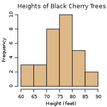
Histogram

In statistics, a histogram is a graphical representation showing a visual impression of the distribution of data. It is an estimate of the probability distribution of a continuous variable and was first introduced by Karl Pearson.^[1] A histogram consists of tabular frequencies, shown as adjacentrectangles, erected over discrete intervals (bins), with an area equal to the frequency of the observations in the interval. The height of a rectangle is also equal to the frequency density of the interval, i.e., the frequency divided by the width of the interval. The total area of the histogram is equal to the number of data. A histogram may also be normalized displaying relative frequencies. It then shows the proportion of cases that fall into each of several categories, with the total area equaling 1. The categories are usually specified as consecutive, non-overlapping intervals of a variable. The categories (intervals) must be adjacent, and often are chosen to be of the same size.^[2] The rectangles of a histogram are drawn so that they touch each other to indicate that the original variable is continuous.^[3]

Histograms are used to plot density of data, and often for density estimation: estimating the probability density function of the underlying variable. The total area of a histogram used for probability density is always normalized to 1. If the length of the intervals on the x-axis are all 1, then a histogram is identical to a relative frequency plot.

An alternative to the histogram is kernel density estimation, which uses a kernel to smooth samples. This will construct a smooth probability density function, which will in general more accurately reflect the underlying variable.

The histogram is one of the seven basic tools of quality control

for example.