| The area of a polygon is the number of square units inside the polygon. Area is 2-dimensional like a carpet or an area rug. | ||
| A parallelogram is a 4-sided shape formed by two pairs of parallel lines. Opposite sides are equal in length and opposite angles are equal in measure. To find the area of a parallelogram, multiply the base by the height. The formula is: | ![[IMAGE]](http://www.mathgoodies.com/lessons/vol1/images/parallelogram.gif) | |
| The base and height of a parallelogram must be perpendicular. However, the lateral sides of a parallelogram are not perpendicular to the base. Thus, a dotted line is drawn to represent the height. Let's look at some examples involving the area of a parallelogram. | ||
| Example 1: | Find the area of a parallelogram with a base of 12 centimeters and a height of 5 centimeters. | ![[IMAGE]](http://www.mathgoodies.com/lessons/vol1/images/parallelogram_5x12_rt.gif) |
| Solution: | ||
| Example 2: | Find the area of a parallelogram with a base of 7 inches and a height of 10 inches. | ![[IMAGE]](http://www.mathgoodies.com/lessons/vol1/images/parallelogram_7x10_rt.gif) |
| Solution: | ||
| Example 3: | The area of a parallelogram is 24 square centimeters and the base is 4 centimeters. Find the height. | ![[IMAGE]](http://www.mathgoodies.com/lessons/vol1/images/parallelogram_4x6_rt.gif) |
| Solution: | ||
| 24 cm2 = (4 cm) · | ||
| 24 cm2 ÷ (4 cm) = | ||
| Summary: | Given the base and height of a parallelogram, we can find the area. Given the area of a parallelogram and either the base or the height, we can find the missing dimension. The formula for area of a parallelogram is: | |
Saturday 29 December 2012
Area of a Parallelogram
Tuesday 25 December 2012
Statistics
Statistics is the study of the collection, organization, analysis, interpretation and presentation of data.[1][2] It deals with all aspects of this, including the planning of data collection in terms of the design of surveys and experiments.[1]
A statistician is someone who is particularly well-versed in the ways of thinking necessary for the successful application of statistical analysis. Such people have often gained experience through working in any of a wide number of fields. There is also a discipline called mathematical statistics that studies statistics mathematically.
The word statistics, when referring to the scientific discipline, is singular, as in "Statistics is an art."[3] This should not be confused with the word statistic, referring to a quantity (such as mean ormedian) calculated from a set of data,[4] whose plural is statistics ("this statistic seems wrong" or "these statistics are misleading").


Mean
In statistics, mean has three related meanings[1] :
- the arithmetic mean of a sample (distinguished from the geometric mean or harmonic mean).
- the expected value of a random variable.
- the mean of a probability distribution.
There are other statistical measures of central tendency that should not be confused with means - including the 'median' and 'mode'. Statistical analyses also commonly use measures ofdispersion, such as the range, interquartile range, or standard deviation. Note that not every probability distribution has a defined mean; see the Cauchy distribution for an example.
For a data set, the arithmetic mean is equal to the sum of the values divided by the number of values. The arithmetic mean of a set of numbers x1, x2, ..., xn is typically denoted by  , pronounced "x bar". If the data set were based on a series of observations obtained by sampling from a statistical population, the arithmetic mean is termed the "sample mean" () to distinguish it from the "population mean" (
 or x).[2] For a finite population, the population mean of a property is equal to the arithmetic mean of the given property while considering every member of the population. For example, the population mean height is equal to the sum of the heights of every individual divided by the total number of individuals.
, pronounced "x bar". If the data set were based on a series of observations obtained by sampling from a statistical population, the arithmetic mean is termed the "sample mean" () to distinguish it from the "population mean" ( or x).[2] For a finite population, the population mean of a property is equal to the arithmetic mean of the given property while considering every member of the population. For example, the population mean height is equal to the sum of the heights of every individual divided by the total number of individuals.
The sample mean may differ from the population mean, especially for small samples. The law of large numbers dictates that the larger the size of the sample, the more likely it is that the sample mean will be close to the population mean.
For a probability distribution, the mean is equal to the sum or integral over every possible value weighted by the probability of that value. In the case of a discrete probability distribution, the mean of a discrete random variable x is computed by taking the product of each possible value of x and its probability P(x), and then adding all these products together, giving  .
.
.Arithmetic mean (AM)
Main article: Arithmetic mean
The arithmetic mean is the "standard" average, often simply called the "mean".

For example, the arithmetic mean of five values: 4, 36, 45, 50, 75 is


The mean may often be confused with the median, mode or range. The mean is the arithmetic average of a set of values, or distribution; however, forskewed distributions, the mean is not necessarily the same as the middle value (median), or the most likely (mode). For example, mean income is skewed upwards by a small number of people with very large incomes, so that the majority have an income lower than the mean. By contrast, the median income is the level at which half the population is below and half is above. The mode income is the most likely income, and favors the larger number of people with lower incomes. The median or mode are often more intuitive measures of such data.
Nevertheless, many skewed distributions are best described by their mean – such as the exponential and Poisson distributions.
Median
statistics and probability theory, median is described as the numerical value separating the higher half of a sample, a population, or a probability distribution, from the lower half. The median of a finite list of numbers can be found by arranging all the observations from lowest value to highest value and picking the middle one. If there is an even number of observations, then there is no single middle value; the median is then usually defined to be the mean of the two middle values.[1][2]
A median is only defined on one-dimensional data, and is independent of any distance metric. A geometric median, on the other hand, is defined in any number of dimensions.
In a sample of data, or a finite population, there may be no member of the sample whose value is identical to the median (in the case of an even sample size); if there is such a member, there may be more than one so that the median may not uniquely identify a sample member. Nonetheless, the value of the median is uniquely determined with the usual definition. A related concept, in which the outcome is forced to correspond to a member of the sample, is the medoid. At most, half the population have values strictly less than the median, and, at most, half have values strictly greater than the median. If each group contains less than half the population, then some of the population is exactly equal to the median. For example, if a < b < c, then the median of the list {a, b, c} is b. If a <> b <> c as well, then only a is strictly less than the median, and only c is strictly greater than the median. Since each group is less than half (one-third, in fact), the leftover b is strictly equal to the median (a truism).
Likewise, if a < b < c < d, then the median of the list {a, b, c, d} is the mean of b and c; i.e., it is (b + c)/2.
The median can be used as a measure of location when a distribution is skewed, when end-values are not known, or when one requires reduced importance to be attached to outliers, e.g., because they may be measurement errors.
In terms of notation, some authors represent the median of a variable x either as  or as
or as  [1] There is no simple, widely accepted standard notation for the median, so the use of these or other symbols for the median needs to be explicitly defined when they are introduced.
or as [1] There is no simple, widely accepted standard notation for the median, so the use of these or other symbols for the median needs to be explicitly defined when they are introduced.Mode
The mode is the value that appears most often in a set of data.
Like the statistical mean and median, the mode is a way of expressing, in a single number, important information about a random variable or a population. The numerical value of the mode is the same as that of the mean and median in a normal distribution, and it may be very different in highly skewed distributions.
The mode is not necessarily unique, since the same maximum frequency may be attained at different values. The most extreme case occurs in uniform distributions, where all values occur equally frequently.
The mode of a discrete probability distribution is the value x at which its probability mass function takes its maximum value. In other words, it is the value that is most likely to be sampled.
The mode of a continuous probability distribution is the value x at which its probability density function has its maximum value, so, informally speaking, the mode is at the peak.
As noted above, the mode is not necessarily unique, since the probability mass function or probability density function may take the same maximum value at several points x1, x2, etc.
The above definition tells us that only global maxima are modes. Slightly confusingly, when a probability density function has multiple local maxima it is common to refer to all of the local maxima as modes of the distribution. Such a continuous distribution is called multimodal (as opposed to unimodal).
In symmetric unimodal distributions, such as the normal (or Gaussian) distribution (the distribution whose density function, when graphed, gives the famous "bell curve"), the mean (if defined), median and mode all coincide. For samples, if it is known that they are drawn from a symmetric distribution, the sample mean can be used as an estimate of the population mode.
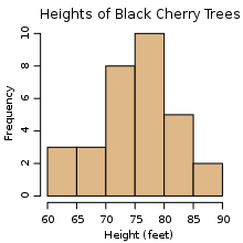
Histogram
In statistics, a histogram is a graphical representation showing a visual impression of the distribution of data. It is an estimate of the probability distribution of a continuous variable and was first introduced by Karl Pearson.[1] A histogram consists of tabular frequencies, shown as adjacentrectangles, erected over discrete intervals (bins), with an area equal to the frequency of the observations in the interval. The height of a rectangle is also equal to the frequency density of the interval, i.e., the frequency divided by the width of the interval. The total area of the histogram is equal to the number of data. A histogram may also be normalized displaying relative frequencies. It then shows the proportion of cases that fall into each of several categories, with the total area equaling 1. The categories are usually specified as consecutive, non-overlapping intervals of a variable. The categories (intervals) must be adjacent, and often are chosen to be of the same size.[2] The rectangles of a histogram are drawn so that they touch each other to indicate that the original variable is continuous.[3]
Histograms are used to plot density of data, and often for density estimation: estimating the probability density function of the underlying variable. The total area of a histogram used for probability density is always normalized to 1. If the length of the intervals on the x-axis are all 1, then a histogram is identical to a relative frequency plot.
An alternative to the histogram is kernel density estimation, which uses a kernel to smooth samples. This will construct a smooth probability density function, which will in general more accurately reflect the underlying variable.
The histogram is one of the seven basic tools of quality control
for example.
Probability
Probability is a measure of the expectation that an event will occur or a statement is true. Probabilities are given a value between 0 (will not occur) and 1 (will occur).[1] The higher the probability of an event, the more certain we are that the event will occur.
The concept has been given an axiomatic mathematical derivation in probability theory, which is used widely in such areas of study as mathematics,statistics, finance, gambling, science, artificial intelligence/machine learning and philosophy to, for example, draw inferences about the expected frequency of events. Probability theory is also used to describe the underlying mechanics and regularities of complex systems.

Interpretations
When dealing with experiments that are random and well-defined in a purely theoretical setting (like tossing a fair coin), probabilities describe the statistical number of outcomes considered divided by the number of all outcomes (tossing a fair coin twice will yield HH with probability 1/4, because the four outcomes HH, HT, TH and TT are possible). When it comes to practical application, however, the word probability does not have a singular direct definition. In fact, there are two major categories of probability interpretations, whose adherents possess conflicting views about the fundamental nature of probability:
- Objectivists assign numbers to describe some objective or physical state of affairs. The most popular version of objective probability is frequentist probability, which claims that the probability of a random event denotes the relative frequency of occurrence of an experiment's outcome, when repeating the experiment. This interpretation considers probability to be the relative frequency "in the long run" of outcomes.[2] A modification of this is propensity probability, which interprets probability as the tendency of some experiment to yield a certain outcome, even if it is performed only once.
- Subjectivists assign numbers per subjective probability, i.e., as a degree of belief.[3] The most popular version of subjective probability is Bayesian probability, which includes expert knowledge as well as experimental data to produce probabilities. The expert knowledge is represented by some (subjective) prior probability distribution. The data is incorporated in a likelihood function. The product of the prior and the likelihood, normalized, results in a posterior probability distribution that incorporates all the information known to date.[4] Starting from arbitrary, subjective probabilities for a group of agents, some Bayesians[who?] claim that all agents will eventually have sufficiently similar assessments of probabilities, given enough evidence.
Etymology
The word Probability derives from the Latin probabilitas, which can also mean probity, a measure of the authority of a witness in a legal case in Europe, and often correlated with the witness'snobility. In a sense, this differs much from the modern meaning of probability, which, in contrast, is a measure of the weight of empirical evidence, and is arrived at from inductive reasoning andstatistical inference.
Theory
Like other theories, the theory of probability is a representation of probabilistic concepts in formal terms—that is, in terms that can be considered separately from their meaning. These formal terms are manipulated by the rules of mathematics and logic, and any results are interpreted or translated back into the problem domain.
There have been at least two successful attempts to formalize probability, namely the Kolmogorov formulation and the Cox formulation. In Kolmogorov's formulation (see probability space), setsare interpreted as events and probability itself as a measure on a class of sets. In Cox's theorem, probability is taken as a primitive (that is, not further analyzed) and the emphasis is on constructing a consistent assignment of probability values to propositions. In both cases, the laws of probability are the same, except for technical details.
There are other methods for quantifying uncertainty, such as the Dempster-Shafer theory or possibility theory, but those are essentially different and not compatible with the laws of probability as usually understood.
[edit]Applications
Probability theory is applied in everyday life in risk assessment and in trade on financial markets. Governments apply probabilistic methods in environmental regulation, where it is called pathway analysis. A good example is the effect of the perceived probability of any widespread Middle East conflict on oil prices—which have ripple effects in the economy as a whole. An assessment by a commodity trader that a war is more likely vs. less likely sends prices up or down, and signals other traders of that opinion. Accordingly, the probabilities are neither assessed independently nor necessarily very rationally. The theory of behavioral finance emerged to describe the effect of such groupthink on pricing, on policy, and on peace and conflict.[12]
The discovery of rigorous methods to assess and combine probability assessments has changed society. It is important for most citizens to understand how probability assessments are made, and how they contribute to decisions.
Another significant application of probability theory in everyday life is reliability. Many consumer products, such as automobiles and consumer electronics, use reliability theory in product design to reduce the probability of failure. Failure probability may influence a manufacture's decisions on a product's warranty.[13]
The cache language model and other statistical language models that are used in natural language processing are also examples of applications of probability theory.
[edit]Mathematical treatment
Consider an experiment that can produce a number of results. The collection of all results is called the sample space of the experiment. The power set of the sample space is formed by considering all different collections of possible results. For example, rolling a die can produce six possible results. One collection of possible results gives an odd number on the die. Thus, the subset {1,3,5} is an element of the power set of the sample space of die rolls. These collections are called "events." In this case, {1,3,5} is the event that the die falls on some odd number. If the results that actually occur fall in a given event, the event is said to have occurred.
A probability is a way of assigning every event a value between zero and one, with the requirement that the event made up of all possible results (in our example, the event {1,2,3,4,5,6}) is assigned a value of one. To qualify as a probability, the assignment of values must satisfy the requirement that if you look at a collection of mutually exclusive events (events with no common results, e.g., the events {1,6}, {3}, and {2,4} are all mutually exclusive), the probability that at least one of the events will occur is given by the sum of the probabilities of all the individual events.[14]
The probability of an event A is written as P(A), p(A) or Pr(A).[15] This mathematical definition of probability can extend to infinite sample spaces, and even uncountable sample spaces, using the concept of a measure.
The opposite or complement of an event A is the event [not A] (that is, the event of A not occurring); its probability is given by P(not A) = 1 - P(A).[16] As an example, the chance of not rolling a six on a six-sided die is 1 – (chance of rolling a six)  . See Complementary event for a more complete treatment.
. See Complementary event for a more complete treatment.
If both events A and B occur on a single performance of an experiment, this is called the intersection or joint probability of A and B, denoted as  .
.
.[edit]Independent probability
If two events, A and B are independent then the joint probability is

for example, if two coins are flipped the chance of both being heads is  [17]
[17]
[17][edit]Mutually exclusive
If either event A or event B or both events occur on a single performance of an experiment this is called the union of the events A and B denoted as  . If two events are mutually exclusive then the probability of either occurring is
. If two events are mutually exclusive then the probability of either occurring is
For example, the chance of rolling a 1 or 2 on a six-sided die is 
[edit]Not mutually exclusive
If the events are not mutually exclusive then

For example, when drawing a single card at random from a regular deck of cards, the chance of getting a heart or a face card (J,Q,K) (or one that is both) is  , because of the 52 cards of a deck 13 are hearts, 12 are face cards, and 3 are both: here the possibilities included in the "3 that are both" are included in each of the "13 hearts" and the "12 face cards" but should only be counted once.
, because of the 52 cards of a deck 13 are hearts, 12 are face cards, and 3 are both: here the possibilities included in the "3 that are both" are included in each of the "13 hearts" and the "12 face cards" but should only be counted once.[edit]Conditional probability
Conditional probability is the probability of some event A, given the occurrence of some other event B. Conditional probability is written  , and is read "the probability of A, given B". It is defined by[18]
, and is read "the probability of A, given B". It is defined by[18]
If  then is formally undefined by this expression. However, it is possible to define a conditional probability for some zero-probability events using a σ-algebra of such events (such as those arising from a continuous random variable).[citation needed]
For example, in a bag of 2 red balls and 2 blue balls (4 balls in total), the probability of taking a red ball is ; however, when taking a second ball, the probability of it being either a red ball or a blue ball depends on the ball previously taken, such as, if a red ball was taken, the probability of picking a red ball again would be
  since only 1 red and 2 blue balls would have been remaining.
then is formally undefined by this expression. However, it is possible to define a conditional probability for some zero-probability events using a σ-algebra of such events (such as those arising from a continuous random variable).[citation needed]For example, in a bag of 2 red balls and 2 blue balls (4 balls in total), the probability of taking a red ball is
; however, when taking a second ball, the probability of it being either a red ball or a blue ball depends on the ball previously taken, such as, if a red ball was taken, the probability of picking a red ball again would be since only 1 red and 2 blue balls would have been remaining.[edit]Summary of probabilities
| Event | Probability |
|---|---|
| A | ![P(A)\in[0,1]\,](http://upload.wikimedia.org/math/1/0/c/10ccd2ab2530f78f898e79ea5a17c862.png) |
| not A | 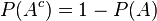 |
| A or B |  |
| A and B |  |
| A given B |  |
[edit]Relation to randomness
Main article: Randomness
In a deterministic universe, based on Newtonian concepts, there would be no probability if all conditions are known, (Laplace's demon). In the case of a roulette wheel, if the force of the hand and the period of that force are known, the number on which the ball will stop would be a certainty. Of course, this also assumes knowledge of inertia and friction of the wheel, weight, smoothness and roundness of the ball, variations in hand speed during the turning and so forth. A probabilistic description can thus be more useful than Newtonian mechanics for analyzing the pattern of outcomes of repeated rolls of roulette wheel. Physicists face the same situation in kinetic theory of gases, where the system, while deterministic in principle, is so complex (with the number of molecules typically the order of magnitude of Avogadro constant 6.02·1023) that only statistical description of its properties is feasible.
Probability theory is required to describe quantum phenomena.[19] A revolutionary discovery of early 20th century physics was the random character of all physical processes that occur at sub-atomic scales and are governed by the laws of quantum mechanics. The objective wave function evolves deterministically but, according to the Copenhagen interpretation, it deals with probabilities of observing, the outcome being explained by a wave function collapse when an observation is made. However, the loss of determinism for the sake of instrumentalism did not meet with universal approval. Albert Einstein famously remarked in a letter[full citation needed] to Max Born: "I am convinced that God does not play dice".[20] Like Einstein, Erwin Schrödinger, whodiscovered the wave function, believed quantum mechanics is a statistical approximation of an underlying deterministic reality.[21] In modern interpretations, quantum decoherence accounts for subjectively probabilistic behavior.
History
The scientific study of probability is a modern development. Gambling shows that there has been an interest in quantifying the ideas of probability for millennia, but exact mathematical descriptions arose much later. There are reasons of course, for the slow development of the mathematics of probability. Whereas games of chance provided the impetus for the mathematical study of probability, fundamental issues are still obscured by the superstitions of gamblers.[6]

According to Richard Jeffrey, "Before the middle of the seventeenth century, the term 'probable' (Latin probabilis) meant approvable, and was applied in that sense, univocally, to opinion and to action. A probable action or opinion was one such as sensible people would undertake or hold, in the circumstances."[7] However, in legal contexts especially, 'probable' could also apply to propositions for which there was good evidence.[8]
Aside from elementary work by Girolamo Cardano in the 16th century, the doctrine of probabilities dates to the correspondence of Pierre de Fermat and Blaise Pascal (1654). Christiaan Huygens (1657) gave the earliest known scientific treatment of the subject.[9] Jakob Bernoulli's Ars Conjectandi (posthumous, 1713) andAbraham de Moivre's Doctrine of Chances (1718) treated the subject as a branch of mathematics.[10] See Ian Hacking's The Emergence of Probability[5] and James Franklin's The Science of Conjecture[full citation needed] for histories of the early development of the very concept of mathematical probability.
The theory of errors may be traced back to Roger Cotes's Opera Miscellanea (posthumous, 1722), but a memoir prepared by Thomas Simpson in 1755 (printed 1756) first applied the theory to the discussion of errors of observation.[citation needed] The reprint (1757) of this memoir lays down the axioms that positive and negative errors are equally probable, and that certain assignable limits define the range of all errors. Simpson also discusses continuous errors and describes a probability curve.
The first two laws of error that were proposed both originated with Pierre-Simon Laplace. The first law was published in 1774 and stated that the frequency of an error could be expressed as an exponential function of the numerical magnitude of the error, disregarding sign. The second law of error was proposed in 1778 by Laplace and stated that the frequency of the error is an exponential function of the square of the error.[11] The second law of error is called the normal distribution or the Gauss law. "It is difficult historically to attribute that law to Gauss, who in spite of his well-known precocity had probably not made this discovery before he was two years old."[11]
Daniel Bernoulli (1778) introduced the principle of the maximum product of the probabilities of a system of concurrent errors.

Adrien-Marie Legendre (1805) developed the method of least squares, and introduced it in his Nouvelles méthodes pour la détermination des orbites des comètes(New Methods for Determining the Orbits of Comets).[citation needed] In ignorance of Legendre's contribution, an Irish-American writer, Robert Adrain, editor of "The Analyst" (1808), first deduced the law of facility of error,
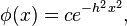
where  is a constant depending on precision of observation, and
  is a scale factor ensuring that the area under the curve equals 1. He gave two proofs, the second being essentially the same as John Herschel's (1850).[citation needed] Gauss gave the first proof that seems to have been known in Europe (the third after Adrain's) in 1809. Further proofs were given by Laplace (1810, 1812), Gauss (1823), James Ivory (1825, 1826), Hagen (1837), Friedrich Bessel (1838), W. F. Donkin (1844, 1856), and Morgan Crofton (1870). Other contributors were Ellis (1844), De Morgan (1864), Glaisher (1872), and Giovanni Schiaparelli (1875). Peters's (1856) formula[clarification needed] for r, the probable error of a single observation, is well known.[to whom?]
is a constant depending on precision of observation, and is a scale factor ensuring that the area under the curve equals 1. He gave two proofs, the second being essentially the same as John Herschel's (1850).[citation needed] Gauss gave the first proof that seems to have been known in Europe (the third after Adrain's) in 1809. Further proofs were given by Laplace (1810, 1812), Gauss (1823), James Ivory (1825, 1826), Hagen (1837), Friedrich Bessel (1838), W. F. Donkin (1844, 1856), and Morgan Crofton (1870). Other contributors were Ellis (1844), De Morgan (1864), Glaisher (1872), and Giovanni Schiaparelli (1875). Peters's (1856) formula[clarification needed] for r, the probable error of a single observation, is well known.[to whom?]
In the nineteenth century authors on the general theory included Laplace, Sylvestre Lacroix (1816), Littrow (1833), Adolphe Quetelet (1853), Richard Dedekind(1860), Helmert (1872), Hermann Laurent (1873), Liagre, Didion, and Karl Pearson. Augustus De Morgan and George Boole improved the exposition of the theory.
Andrey Markov introduced[citation needed] the notion of Markov chains (1906), which played an important role in stochastic processes theory and its applications. The modern theory of probability based on the measure theory was developed by Andrey Kolmogorov (1931).[citation needed]
On the geometric side (see integral geometry) contributors to The Educational Times were influential (Miller, Crofton, McColl, Wolstenholme, Watson, and Artemas Martin).[citation needed]
Subscribe to:
Posts (Atom)